Bresenham's line algorithm: An exploration

Introduction

I have recently been working on a pixel art editor. This editor includes a variety of tools, one of which is a tool for drawing straight lines. Bresenham's line algorithm is often used for line-drawing in pixel art. This post explains why this is, how the algorithm works, and a variation that you might prefer to use.

Line-drawing and rasterisation

In a vector graphics editor, a line drawn by the user is represented mathematically. It always appears smooth regardless of the current magnification level. In a raster graphics editor, the image consists of discrete pixels that you can see when you magnify it:

When the user draws a line in a raster graphics editor, it needs to be rasterised to know which pixels to fill. Often the aim is to produce a smooth result and so anti-aliasing is applied as part of the process. The user might also want to be able to draw lines that start and end on fractional coordinates. Pixel art is different: we prefer the jagged look of non- anti-aliased rasterisation. Thus lines are drawn from whole pixel to whole pixel.

Bresenham's line algorithm is often used when the non-anti-aliased look is desired. Jack Elton Bresenham invented it in 1962. The algorithm does not accept or output fractional coordinate values. This results in lines with the desired jaggies. The algorithm also uses only integer operations. This was useful in the 60s when floating point operations were either not available or were expensive to perform. The following animation shows the algorithm's result for a variety of lines:

A worked example

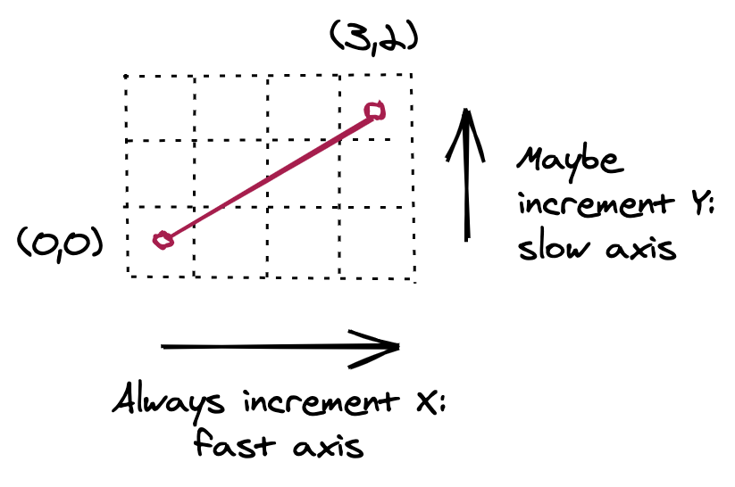
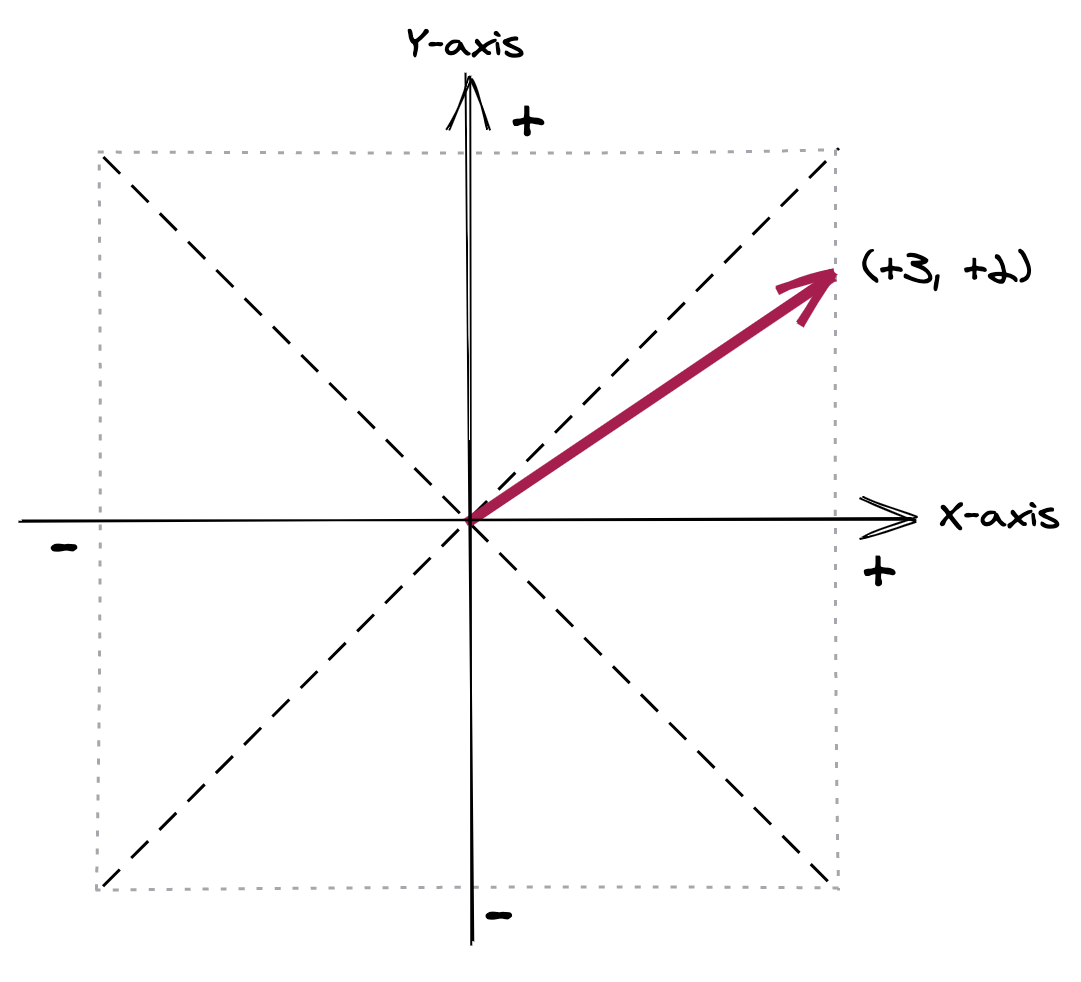
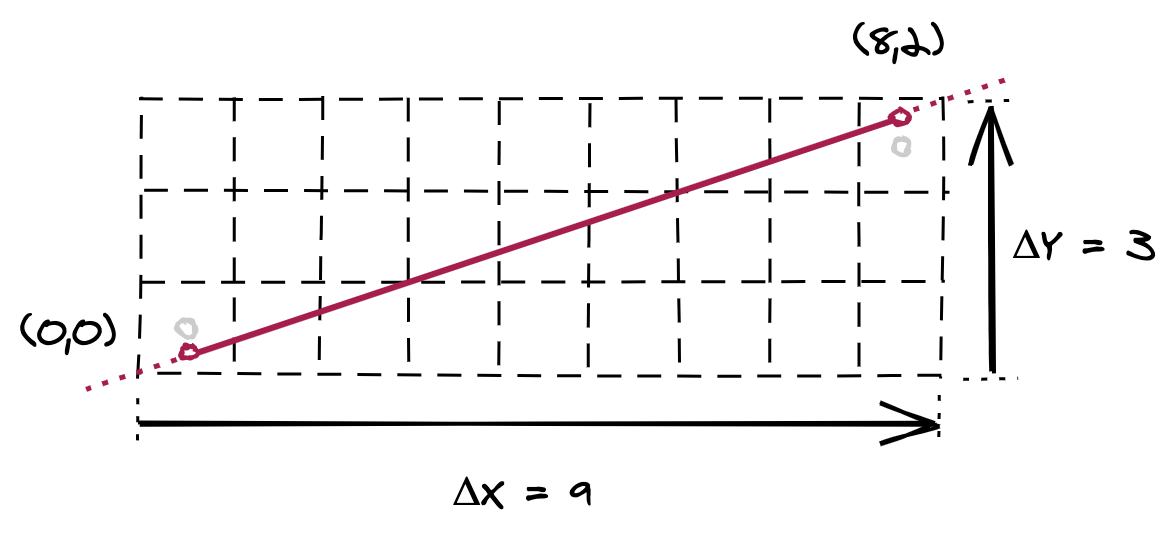
The explanations available on the Web usually focus on deriving the equation that underlies it. I found it more useful to work through an example rasterisation. The line that we will rasterise is the following:

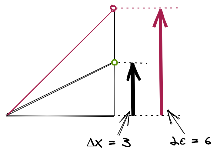
In rasterising this line, we will always be incrementing the X-axis coordinate. We will only sometimes be incrementing the Y-axis coordinate. This is because the change in X, which is 3, is greater than the change in Y, which is 2. The change in X is termed delta X (ΔX) and the change in Y is termed delta Y (ΔY). We are using the Bresenham line algorithm is to answer one question: when should we increment the Y-axis coordinate value?

The 'always' axis is called the fast axis and the 'sometimes' axis is called the slow axis:

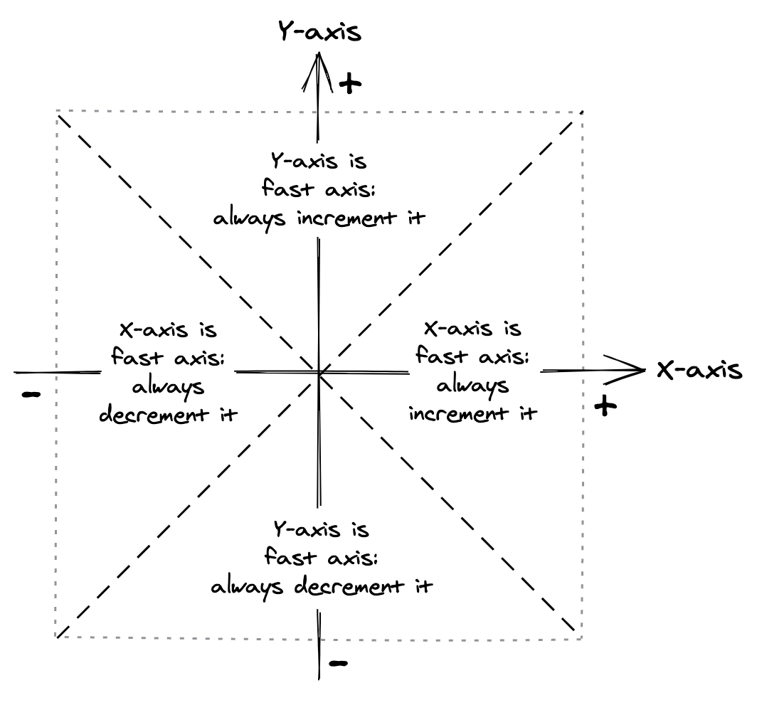
Depending on the line, it is not always the case that the X-axis is the fast axis and the Y-axis is the slow axis. The following diagram shows how the fast axis classification depends upon the directional vector of the line. This also determines whether we need to increment or decrement the fast axis coordinate value:

The following diagram shows how the slow axis classification also depends on the directional vector of the line. It also determines whether we need to sometimes increment or sometimes decrement the slow axis coordinate value:

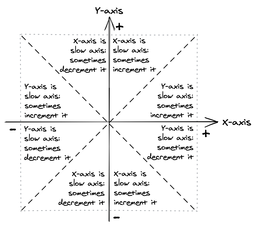
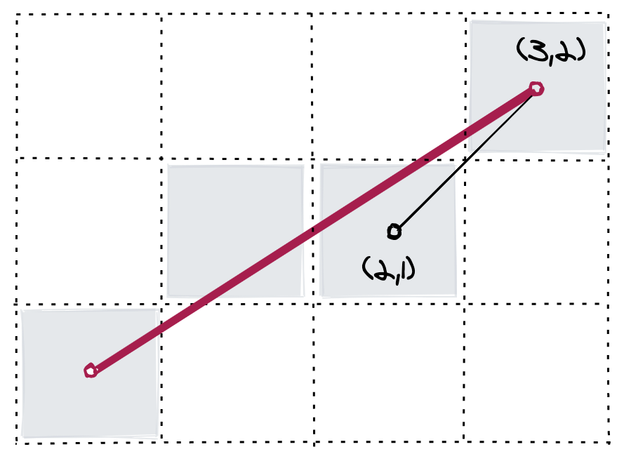
The following is the directional vector of the example line:

It confirms that the X-axis is the fast axis and the Y-axis is the slow axis.

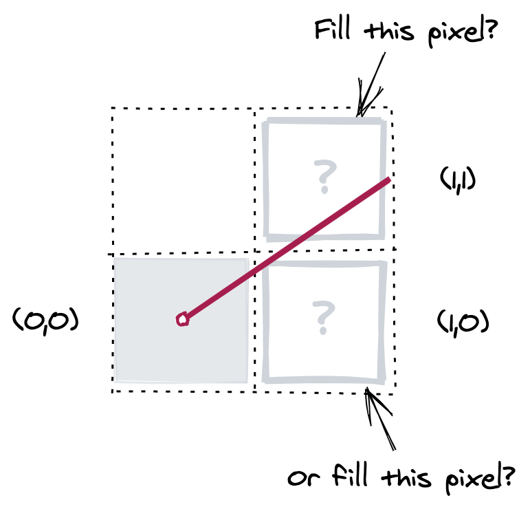
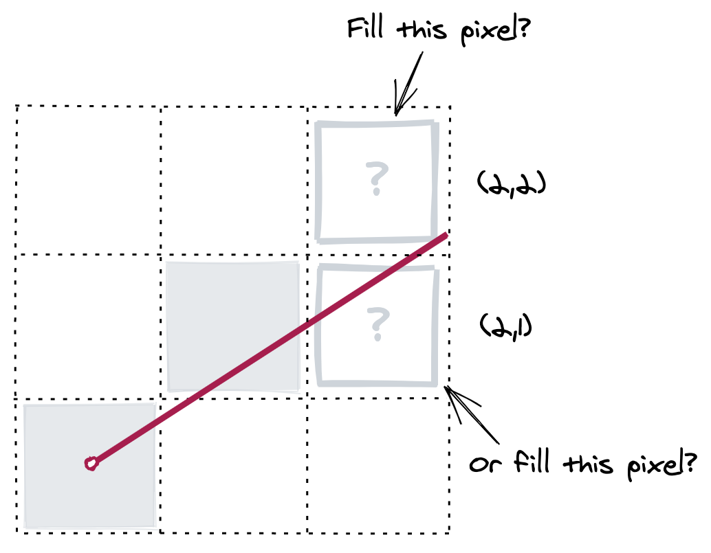
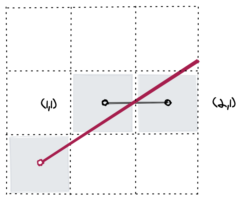
Having classified the axes, we can start the rasterisation process. The first step is easy: the pixel at the start of the line is always filled. For the example line, this is the pixel at (0, 0). The problem now is to determine the next pixel to be filled. We know that the next X-axis coordinate value is 1 because the X-axis is the fast axis. For the Y-axis, we either do or do not increment its coordinate value. This gives us a choice between two possible pixels to fill: the pixel at (1, 0) or the pixel at (1, 1).

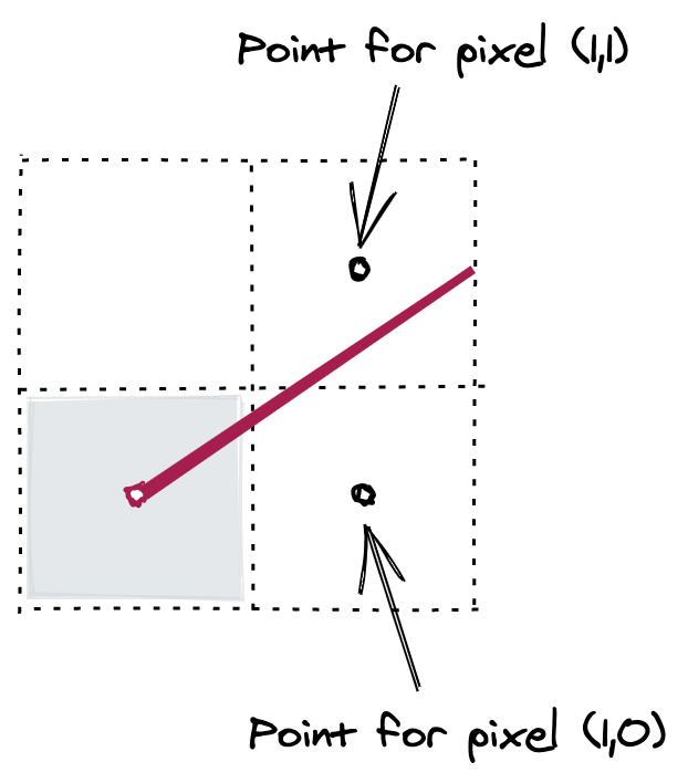
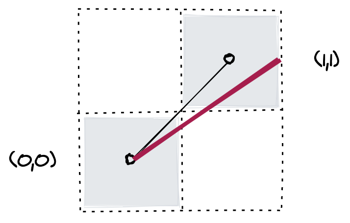
It is possible to think of each pixel as being a point rather than a square. If we do this then we can see that the line passes somewhere between the two possible pixels:

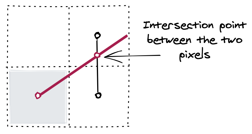
The aim is to determine which of the two pixels is the pixel that the line is closest to when it passes between them. If we draw a line between those two pixels then the line we are rasterising will intersect it at some point:

The midpoint of the line between the two pixels is of course exactly between them:

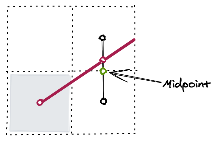
We can now define a rule: only increment the Y coordinate value if the intersection point is equal to or above the midpoint. In this example, the intersection point is above the midpoint. We know to fill the pixel at (1, 1) rather than the pixel at (1, 0).

How do we express this mathematically? We could put exact figures into the calculation:

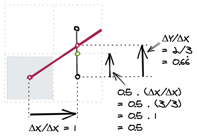
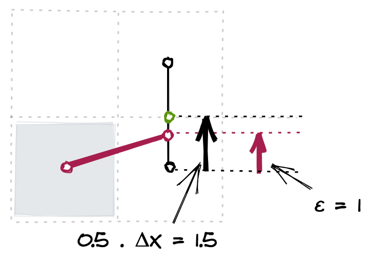
The problem is that we will almost certainly end up with floating point values. Remember, a key feature of the Bresenham algorithm is it uses only integer operations. We can avoid such values if we instead use the rate of change of the fast axis as the relative unit in our calculations. The rate of change of the fast axis is ΔX. Thus the distance between the two pixels is ΔX, the midpoint is half of that, and the intersection point is ΔY above the starting pixel:

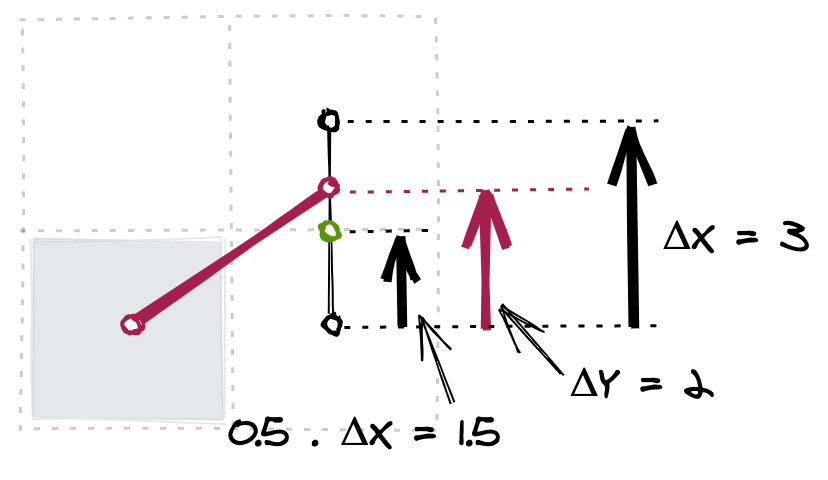
(Note that there is a floating point value in the above diagram — 1.5 — but I will show how to avoid it in our calculations.)

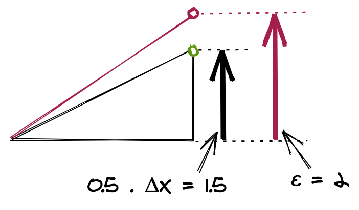
We will use epsilon, with symbol ε, to represent the current rate of change in Y. This is because the rate of change will not always be ΔY. It can vary depending on any error in each iteration of the algorithm. The initial value for ε is zero, and at the start of each iteration we will add ΔY to it. This addition represents the change in Y that occurs each time we take one step along the X-axis. Since we are currently in the first iteration of the algorithm, we add ΔY to ε and so the new value of ε is 0 + 2 which is 2.

We can now compare the value of ε to the value of the midpoint:

To avoid a floating point value here, we can multiply both values by two before comparing them. By doing this we are comparing 2ε (4) to ΔX (3):

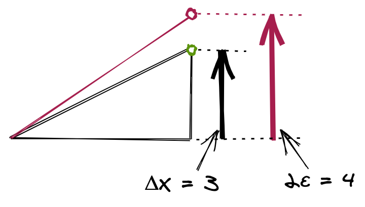
The value of ε is greater than the midpoint value, so we know to increment the Y-axis coordinate value. We fill the pixel at (1, 1):

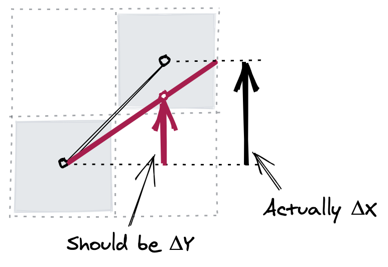
We determined that the intersection point was closer to the pixel at (1, 1). But that point did not fall exactly on the pixel's point. This means that by filling the pixel at (1, 1), the change in Y is ΔX rather than ΔY:

Each iteration of the algorithm works relative to the pixel filled in the last iteration. Since we are about to start a new iteration, we need to adjust the value of ε so that it is relative to the pixel just filled. We incremented the Y-coordinate value, so the change in Y was ΔX and thus we can adjust ε by subtracting ΔX from it. This is 2 - 3 which equals -1 and so this is the new value of ε:

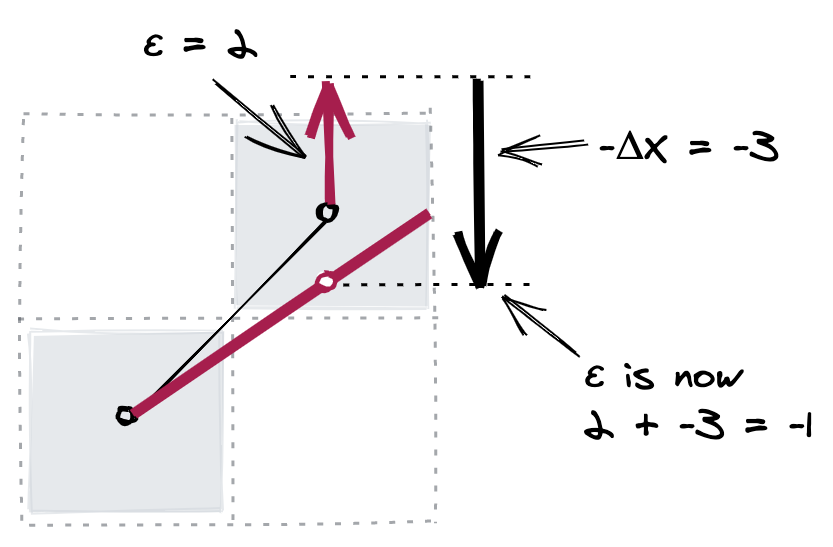
This new value for ε shows that the true intersection point was below the filled pixel. This is correct.

We can now begin the next iteration of the algorithm:

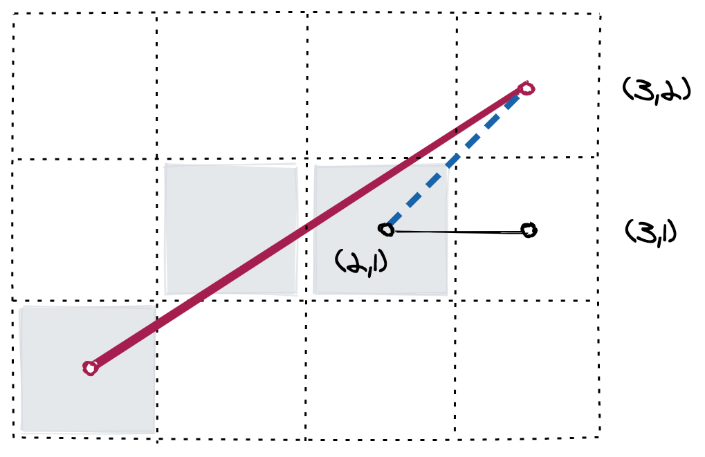
As before we have to determine if the Y coordinate value should or should not be incremented. And as before we first add ΔY to ε. Since the value of ε after the last iteration was -1, the new value of ε is 1. We use this value in our diagram to find the intersection point between the two possible pixels:

The line we are checking is actually the line that extends from the pixel we last filled to the point at which the line we are rasterising passes between the two possible pixels. I have shown this as the blue dashed line in the following diagram:

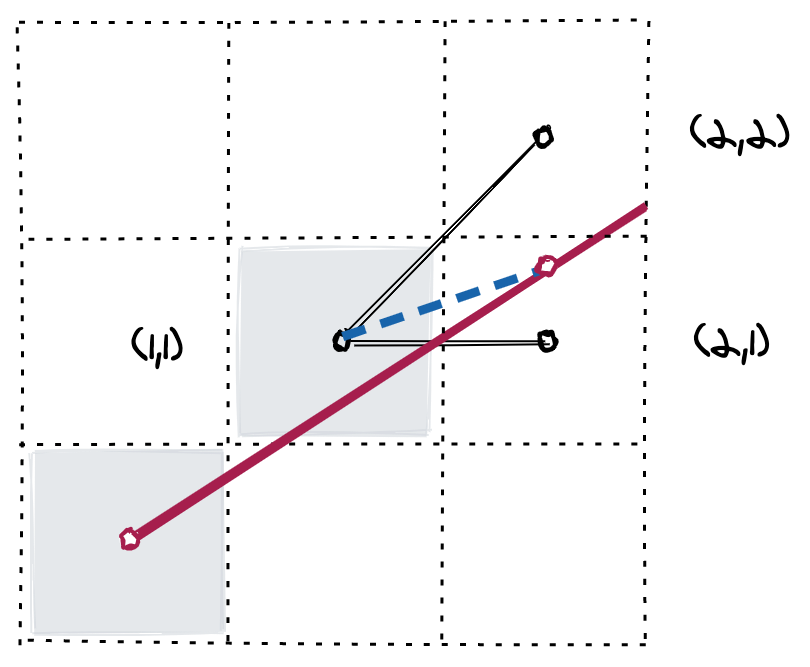
Again, to avoid a floating point value, we can multiply both values by two so that we are comparing 2ε (2) to ΔX (3):

Since the intersection point is not above the midpoint, we do not increment Y and so it is pixel (2, 1) that is filled.

Because we did not increment Y, the value of ε is still relative to the pixel that was just filled. We do not need to adjust it in the way that we did after filling the previous pixel.

Now we can determine the final pixel to fill:

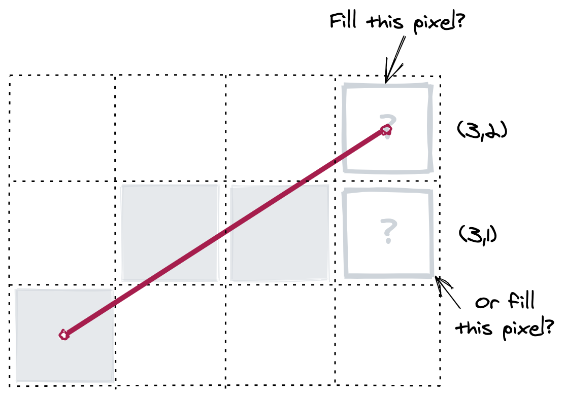
(The pixel to fill is obviously (3, 2) but it is useful for illustrative purposes to continue.)

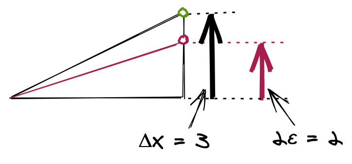
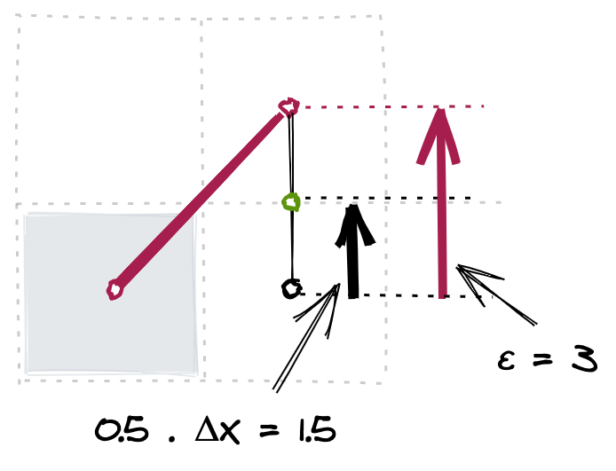
Since we are starting a new iteration of the algorithm, we have to first add ΔY to ε. The value of ε after the last iteration was 1 so the new value of ε is 3.

As before, we need to determine which pixel the line to rasterise is closest to:

And as before, the line we are checking is actually the line that extends from the pixel we last filled to the point at which the line we are rasterising passes between the two possible pixels. I have shown this as the blue dashed line in the following diagram:

As before, we multiply the values by 2 when comparing them:

The value of ε is greater than the threshold so the final pixel to be filled is (3, 2) rather than (3, 1):

And with that the rasterisation of the example line is complete.

An implementation in JavaScript

Below is a JavaScript implementation of the algorithm. It is a variation on the implementation in the node-bresenham package created by the GitHub user madbence:

function bresenham(x0, y0, x1, y1) {
  var arr = [];
  var dx = x1 - x0;
  var dy = y1 - y0;
  var adx = Math.abs(dx);
  var ady = Math.abs(dy);
  var sx = dx > 0 ? 1 : -1;
  var sy = dy > 0 ? 1 : -1;
  var eps = 0;
  if (adx > ady) {
    for (var x = x0, y = y0; sx < 0 ? x >= x1 : x <= x1; x += sx) {
      arr.push({ x: x, y: y });
      eps += ady;
      if (eps << 1 >= adx) {
        y += sy;
        eps -= adx;
      }
    }
  } else {
    for (var x = x0, y = y0; sy < 0 ? y >= y1 : y <= y1; y += sy) {
      arr.push({ x: x, y: y });
      eps += adx;
      if (eps << 1 >= ady) {
        x += sx;
        eps -= ady;
      }
    }
  }
  return arr;
}

Let us see how this compares to the steps followed in the worked example from the previous section.

The inputs to the function are the X and Y coordinates for the start and end points. The return value is an array of coordinate objects that show which pixels should be filled.

Six constants are defined in the initial lines of the function. Firstly, ΔX (dx), ΔY (dy) and the absolute version of each (adx and ady) are defined:

var dx = x1 - x0;
var dy = y1 - y0;
var adx = Math.abs(dx);
var ady = Math.abs(dy);

Then two sign constants are defined:

var sx = dx > 0 ? 1 : -1;
var sy = dy > 0 ? 1 : -1;

The value of sx ('sign X') indicates if ΔX is positive (when sx is 1) or negative (when sx is -1). The value of sy ('sign Y') indicates if ΔY is positive (when sy is 1) or negative (when sy is -1).

The epsilon variable, called eps, is defined next. As expected it is initialised to zero:

var eps = 0;

The algorithm now branches depending on whether the fast axis is the X-axis or the Y-axis. This is found by comparing the values of adx and ady, as shown in the following diagram:

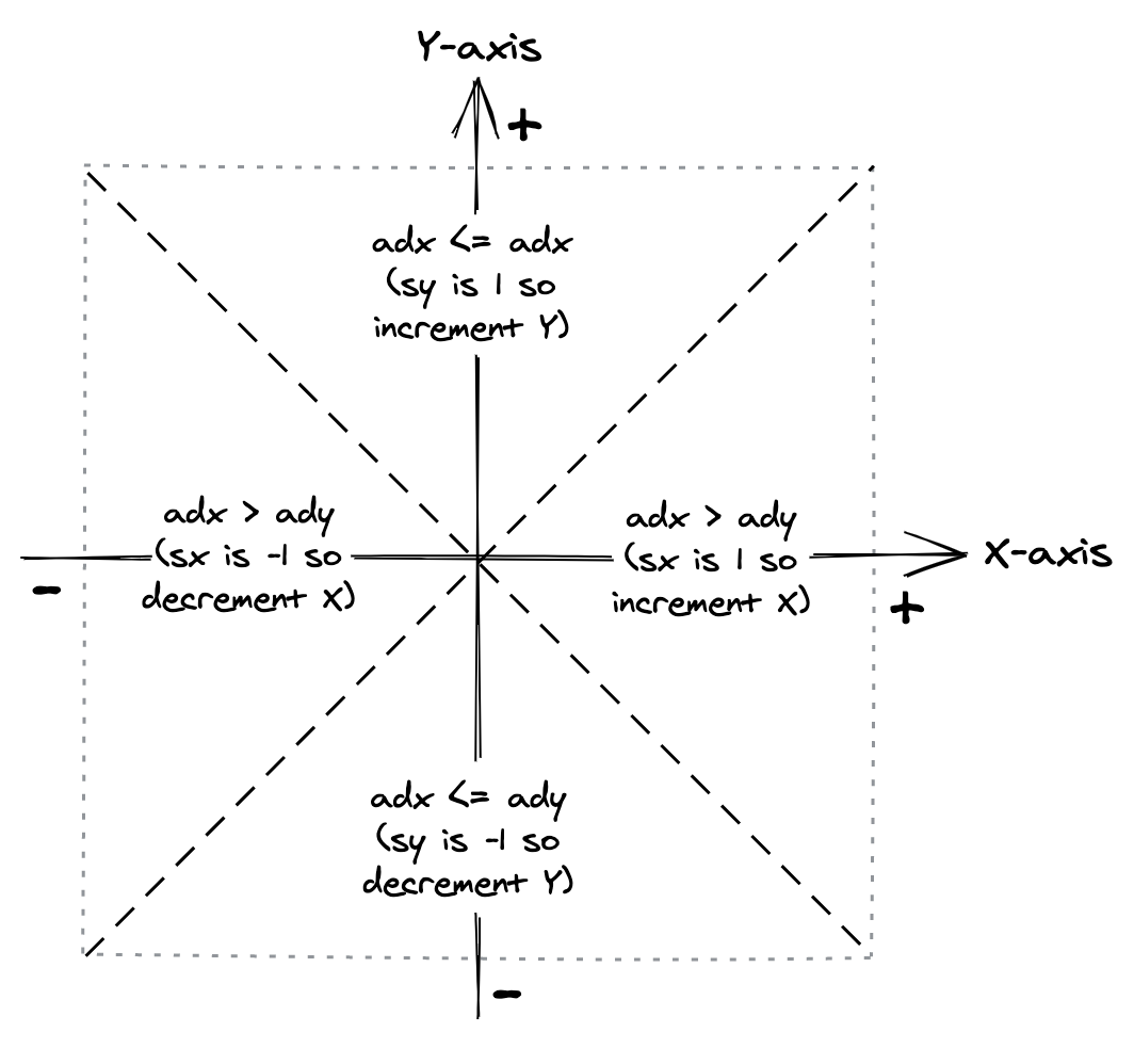
The diagram also shows that if the fast axis is the X-axis then the value of sx shows us if the X coordinate value should be incremented or decremented. If the fast axis is the Y-axis then it is the value of sy that is used to show this for the Y coordinate value.

Let us consider the scenario where the X-axis is the fast axis. The for-loop that executes is the following:

for (var x = x0, y = y0; sx < 0 ? x >= x1 : x <= x1; x += sx) {
  arr.push({ x: x, y: y });
  eps += ady;
  if (eps << 1 >= adx) {
    y += sy;
    eps -= adx;
  }
}

The variables x and y identify the next pixel to be filled. The variable x is initialised to the line's starting X value. It is always incremented if ΔX is positive or always decremented if ΔX is negative, until x1 is reached. The variable y is initialised to the line's starting Y value. At the start of each iteration of the loop, x and y are pushed to the result array:

arr.push({ x: x, y: y });

Then the absolute value of ΔY is added to ε:

eps += ady;

Then the value of ε is tested to see if it is equal to or above the absolute midpoint value of 0.5 × ΔX. To avoid a possible floating point value, this compares 2ε to ΔX:

if (eps << 1 >= adx)

(The expression eps << 1 has the effect of multiplying ε by 2.)

If this condition tests as true then two actions occur. The value of y is incremented or decremented (according to the directional vector of the line):

y += sy;

Then the absolute value of ΔX is subtracted from ε:

eps -= adx;

This iteration of the for-loop is now complete. The loop continues until the end of the line is reached, at which point the result array is returned.

You should recognise these steps from the worked example in the previous section. The difference is that this implementation deals with all possible directional vectors. As a result and to minimise code repetition, the calculations use sx, sy, and the absolute versions of ΔX and ΔY.

Observing the results

For many lines the rasterisation result is good. For example, the following is the result of rasterising a line where ΔX and ΔY are equal:

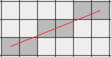
A line from (0, 0) to (5, 2) rasterises well, with an increment in Y for every second increment in X:

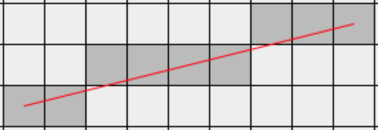
I expected a similar even stepping for a line from (0, 0) to (8, 2). This could be rasterised as an increment in Y for every third increment in X. But this is not the case:

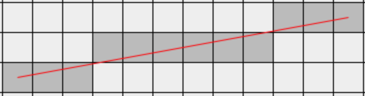
The situation is similar for a line from (0, 0) to (11, 2). This could be rasterised as an increment in Y for every fourth increment in X, but again this is not the case:

Finally here is a line from (0, 0) to (14, 2). I would prefer it to be rasterised as an increment in Y for every fifth increment in X:

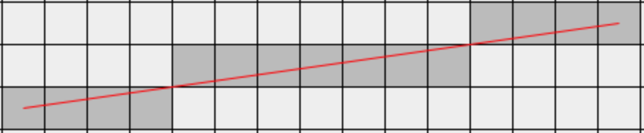
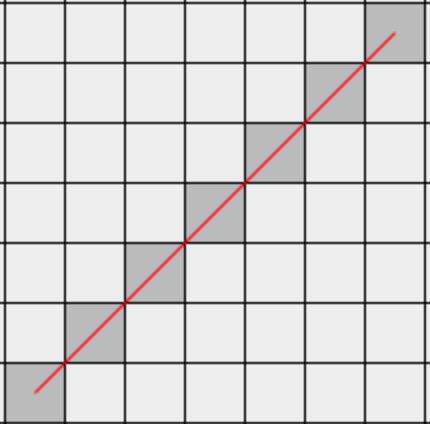
The Bresenham line algorithm rasterises a line that extends from the centre of the starting pixel to the centre of the ending pixel. This is shown as the red line in each of the above rasterisation images. To change the rasterisation result, we would need to change this imaginary line somehow. If we want to rasterise a line from (0, 0) to (8, 2) as an increment in Y for every third increment in X, we would need a different line:

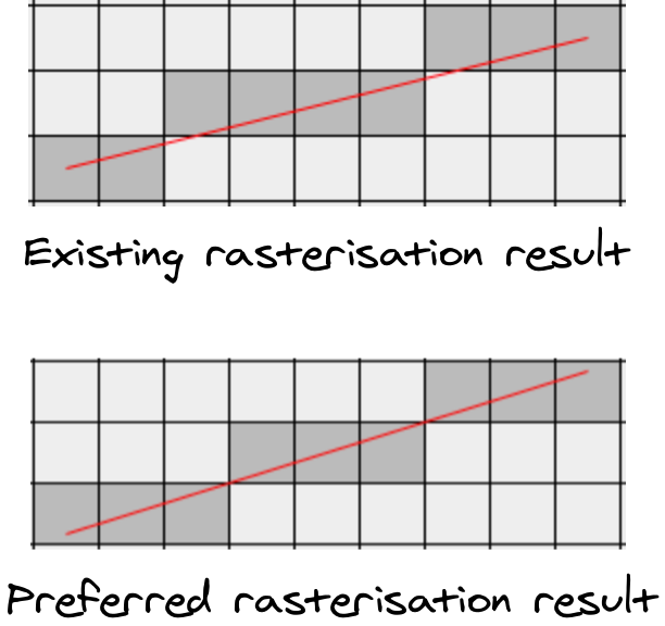
This new line has two differences compared to the existing line:

1. It has a steeper gradient.
2. The start of the line is at a point below the centre of the starting pixel.

Let us now calculate some values for these differences. The new line has ΔX and ΔY values that are each one greater than those of the existing line:

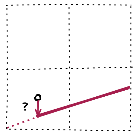
With the existing line, the ε (epsilon) value gets initialised to zero. This is because the starting point of the line is at the centre of the starting pixel. For the new line, the initial value of ε needs to be some negative value. This would position the starting point of the line below the centre of the starting pixel:

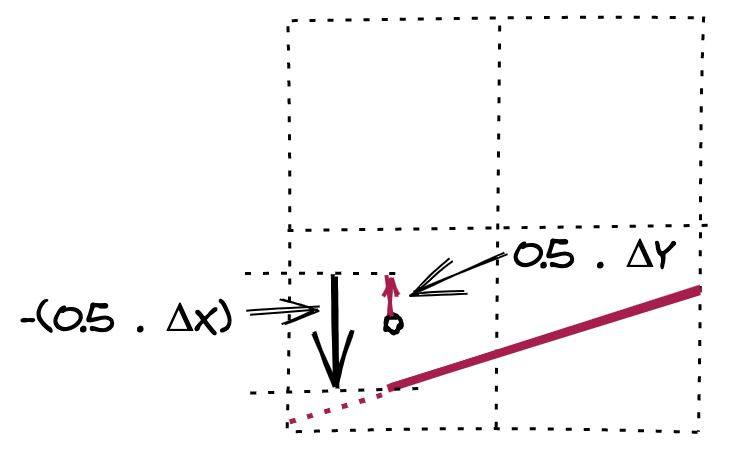
We represent the change in X of each pixel increment as ΔX and the change in Y as ΔY. The change in X at the starting point is 0.5 × ΔX and the change in Y is 0.5 × ΔY:

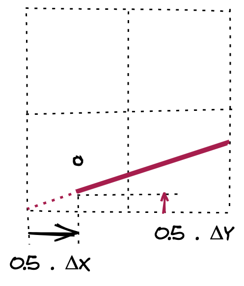
We need the change in Y to be relative to the centre of the pixel. This is the value that we will initialise ε to. We can calculate this by subtracting 0.5 × ΔX from 0.5 × ΔY:

This can be rewritten as (ΔY - ΔX) × 0.5.

Now we have expressions for these differences. We can take the Bresenham line algorithm and update it to the following:

function bresenhamVariation(x0, y0, x1, y1) {
  var arr = [];
  var dx = x1 - x0;
  var dy = y1 - y0;
  var adx = (Math.abs(dx) + 1) << 1;
  var ady = (Math.abs(dy) + 1) << 1;
  var sx = dx > 0 ? 1 : -1;
  var sy = dy > 0 ? 1 : -1;
  if (adx > ady) {
    var eps = (ady - adx) >> 1;
    for (var x = x0, y = y0; sx < 0 ? x >= x1 : x <= x1; x += sx) {
      arr.push({ x: x, y: y });
      eps += ady;
      if (eps << 1 >= adx) {
        y += sy;
        eps -= adx;
      }
    }
  } else {
    var eps = (adx - ady) >> 1;
    for (var x = x0, y = y0; sy < 0 ? y >= y1 : y <= y1; y += sy) {
      arr.push({ x: x, y: y });
      eps += adx;
      if (eps << 1 >= ady) {
        x += sx;
        eps -= ady;
      }
    }
  }
  return arr;
}

The changes are minimal. I add one to adx and ady to increase the line gradient, but I also multiply these values by 2:

var adx = (Math.abs(dx) + 1) << 1;
var ady = (Math.abs(dy) + 1) << 1;

The calculation of the initial value of ε requires multiplying by one half. To avoid a potential floating point value here I double adx and ady.

The final change I made is that the initial value of ε now depends on whether the fast axis is the X-axis or the Y-axis:

if (adx > ady) {
  // The X-axis is the fast axis.
  var eps = (ady - adx) >> 1;

  // for-loop here
} else {
  // The Y-axis is the fast axis.
  var eps = (adx - ady) >> 1;

  // for-loop here
}

I have embedded a simple interactive visualisation below. You can use it to compare lines from the original algorithm with lines from the altered algorithm. Click on a square to draw a line from the center of the visualisation to that pixel. Use the dropdown to select the algorithm.

Conclusion

The Bresenham line algorithm may have been invented many years ago but it is still relevant today. I have been able to create a variation that suits my particular needs for line rasterisation.

---

Changelog

• 2020-07-30 Initial version
• 2020-08-03 Some wording and image changes
• 2020-08-27 Plain English improvements

# Comments

Comments on this site are implemented using GitHub Issues. To add your comment, please add it to this GitHub Issue. It will then appear below.